Assignment Code: MCS-211/TMA/2024

Course Code: MCS-211

Assignment Name: Design and Analysis of Algorithm

Year: 2024

Verification Status: Verified by Professor

Q1. a) Develop an efficient algorithm to find a list of prime numbers from 100 to 1000.

Ans) Algorithm to find a list of prime numbers from 100 to 100 efficiently.

a) Initialize a List of Potential Primes: Create a list containing all numbers from 100 to 1000.

b) Identify Composite Numbers: Start with the smallest prime number (2) and mark all its multiples in the list as composite (not prime). Then move to the next unmarked number and repeat the process until you reach the square root of 1000.

c) Collect Prime Numbers: Iterate through the list, and all unmarked numbers are primes. Collect these prime numbers.

Here's a Python implementation based on the above steps:

def find_primes(start, end):

# Initialize a list containing all numbers from start to end

primes = [True] * (end + 1)

primes[0:2] = [False, False] # 0 and 1 are not primes

# Mark multiples of each prime as composite

for p in range(2, int(end ** 0.5) + 1):

if primes[p]:

for i in range(p * p, end + 1, p):

primes[i] = False

# Collect prime numbers from the list

prime_numbers = [i for i in range(start, end + 1) if primes[i]]

return prime_numbers

# Find prime numbers from 100 to 1000

primes_from_100_to_1000 = find_primes(100, 1000)

print(primes_from_100_to_1000)

This algorithm efficiently finds prime numbers within the specified range by eliminating multiples of each prime number, leading to a list of prime numbers from 100 to 1000.

Q1. b) Differentiate between Polynomial-time and exponential-time algorithms. Give an example of one problem each for these two running times.

Ans) Difference between Polynomial-time algorithms and Exponential-time algorithms is as follows:

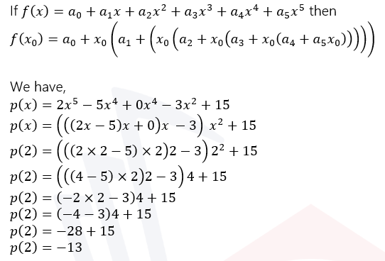
Q1. c) Using Horner’s rule, evaluate the polynomial p(x)=2x^5-5x^4-3x^2+15 at x=2. Analyse, the computation time required for polynomial evaluation using Horner’s rule against the Brute force method.

Ans) Horner's rule for polynomial

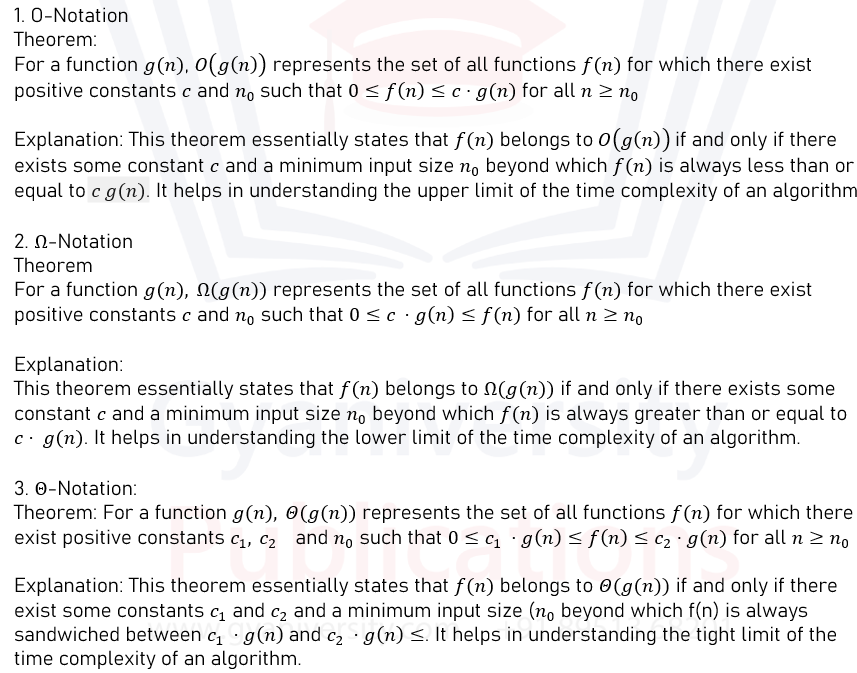
Q1. d) State and explain the theorems for computing the bounds O, π and Θ. Apply these theorem to find the O-notation, Ω-notation and Θ-notation for the function: f(n)=10n^3+18n^2+1

Ans) Theorems for computing the bounds O, π and Θ

Q1. e) Explain binary exponentiation for computing the value 5^19, Write the right-to-left binary exponentian algorithm and show its working for the exponentian 5^19. Also, find the worst-case complexity of this algorithm.

Ans) Binary exponentiation is an algorithm used to efficiently compute the power of a number raised to a non-negative integer exponent. It works by breaking down the exponent into its binary representation, allowing for more efficient computation through repeated squaring.

The right-to-left binary exponentiation algorithm, also known as the modular exponentiation algorithm, is a variant of binary exponentiation that iterates through the binary digits of the exponent from right to left. This algorithm is particularly useful when dealing with large exponents or modular arithmetic operations.

Here's how the right-to-left binary exponentiation algorithm works:

1. Initialize the result = 1

2. Convert the exponent b to its binary representation.

3. Iterate through the binary digits of b from right to left:

- For each binary digit d of b

- Square the current value of result

- If d is 1, multiply result by the base a

4. After iterating through all binary digits of b, the final value of result is the desired result a^b

The right-to-left binary exponentiation algorithm in Python for computing 5^19

def right_to_left_binary_exponentiation(base, exponent):

result = 1

# Convert the exponent to its binary representation

binary_exponent = bin(exponent)[2:]

# Iterate through the binary digits of the exponent from right to left

for digit in binary_exponent[::-1]:

# Square the current value of result

result = (result result) % (10*9 + 7) # For large numbers, take modulo

# If the current binary digit is 1, multiply result by the base

if digit == '1':

result = (result base) % (10*9 + 7) # For large numbers, take modulo

return result

# Compute 5^19 using right-to-left binary exponentiation

base = 5

exponent = 19

result = right_to_left_binary_exponentiation(base, exponent)

print("Result:", result)

Worst-case complexity

The worst-case complexity of this algorithm is O(log n), where n is the value of the exponent. This is because the algorithm iterates through the bits of the binary exponent, and the number of iterations required is proportional to the number of bits in the exponent, which is logarithmic in the value of the exponent itself.

Q1. f) Write and explain the linear search algorithm and discuss its best and worst-case time complexity. Show the working of the linear search algorithm for the data: 12, 11, 3, 9, 15, 20, 18, 19, 13, 8, 2, 1, 16.

Ans)

Linear Search Algorithm

Linear search, also known as sequential search, is a simple searching algorithm that sequentially checks each element in a list or array until a match is found or the entire list has been searched. It starts at the beginning of the data structure and compares each element with the target value until either the target value is found or the end of the data structure is reached.

Explanation of the linear search algorithm:

1. Start from the first element in the list.

2. Compare the target value with the current element.

3. If the current element is equal to the target value, return its index.

4. If the current element is not equal to the target value, move to the next element.

5. Repeat steps 2-4 until either the target value is found or the end of the list is reached.

6. If the target value is not found after searching through all elements, return a message indicating the absence of the target value.

Time Complexity:

Best Case:

The best-case scenario occurs when the target element is found at the beginning of the list. In this case, the algorithm would have a time complexity of O(1) because it would only require one comparison.

Worst Case

The worst-case scenario occurs when the target element is either not present in the list or present at the end of the list. In this case, the algorithm would have to traverse through all elements of the list, resulting in a time complexity of O(n), where n is the number of elements in the list.

Linear search algorithm for the given data

Data: 12, 11, 3, 9, 15, 20, 18, 19, 13, 8, 2, 1, 16

Target value: 9

1. Start from the first element: 12

- 12 is not equal to the target value (9), move to the next element.

2. Second element: 11

- 11 is not equal to the target value (9), move to the next element.

3. Third element: 3

- 3 is not equal to the target value (9), move to the next element.

4. Fourth element: 9

- 9 is equal to the target value (9), Return the index of 9, which is 3.

The linear search algorithm successfully found the target value 9 at index 3.

Q1. g) What is a recurrence relation? Solve the following recurrence relations using the Master's method.

Ans) A recurrence relation is a mathematical equation that recursively defines a sequence or a function in terms of its previous values. It expresses the value of a function at a certain point in terms of its value(s) at one or more previous points. Recurrence relations are often used to describe iterative processes or dynamic programming algorithms.

Master theorem is used to solve the recurrence relation of the form:

2. By using Master theorem

Q2. a) What is a Greedy Approach to Problem-solving? Formulate the fractional Knapsack Problem as an optimisation problem and write a greedy algorithm to solve this problem. Solve the following fractional Knapsack problem using this algorithm. Show all the steps.

Suppose there is a knapsack of capacity 15 Kg and 6 items are to packed in it. The weight and profit of the items are as under:

Ans) Greedy approach is a problem-solving strategy that involves making the locally optimal choice at each step with the hope that this choice will lead to a globally optimal solution. In other words, a greedy algorithm makes the best decision at each step without considering the consequences of this decision on future steps. The decision is made based solely on the current state of the problem.

Key characteristics of a greedy approach include:

1. Greedy Choice Property: At each step, a greedy algorithm selects the most advantageous option available, without considering the global context or the future consequences of that decision.

2. Optimal Substructure: The problem must exhibit optimal substructure, meaning that an optimal solution to the problem contains optimal solutions to its subproblems.

3. Doesn't Always Guarantee the Optimal Solution: While greedy algorithms are often simple and efficient, they do not always guarantee the globally optimal solution. However, in many cases, they provide a reasonably good approximation of the optimal solution.

Problem Formulation

The fractional Knapsack Problem can be formulated as an optimization problem as follows:

Given:

n items, each with a weight w_i and a profit p_i.

A knapsack with a weight capacity W.

Objective:

Maximize the total profit obtained by selecting items to pack into the knapsack.

Constraints:

The total weight of selected items cannot exceed the capacity of the knapsack.

Greedy algorithm

Greedy algorithm to solve the fractional Knapsack Problem is as follows:

Calculate the value-to-weight ratio for each item.

Sort the items by value-to-weight ratio in descending order.

Initialize the total profit obtained and the remaining capacity of the knapsack.

Iterate through the sorted list of items:

If the weight of the current item is less than or equal to the remaining capacity of the knapsack, take the entire item and update the total profit and remaining capacity accordingly.

If the weight of the current item exceeds the remaining capacity of the knapsack, take a fraction of the item to fill the remaining capacity and update the total profit accordingly.

Return the maximum total profit obtained.

To solve the fractional Knapsack problem using a greedy algorithm

Calculate the value-to-weight ratio for each item.

Sort the items by value-to-weight ratio in descending order.

Iterate through the sorted list of items, adding items to the knapsack until its capacity is filled.

If an item cannot fit entirely, take a fraction of it to fill the remaining capacity.

Calculate the total profit obtained.

Given:

- Knapsack capacity: 15 Kg

- Number of items: 6

- Profits of items: p = [3, 2, 4, 5, 1, 6]

- Weights of items: w = [2, 1, 2, 1, 5, 1]

Let's proceed with the calculations:

1. Calculate the value-to-weight ratio for each item:

Value-to-weight ratios:

3/2=1.5

2/1=2

4/2=2

5/1=5

1/5=0.2

6/1=6

2. Sort the items by value-to-weight ratio in descending order:

3. Pack items into the knapsack until its capacity is filled:

Initially, the capacity of the knapsack is 15 Kg.

- We start packing items in the sorted order until the knapsack is full or all items are packed.

2. b) What is the purpose of using Huffman Codes? Explain the steps of building a huffman tree. Design the Huffman codes for the following set of characters and their frequencies : a:15, e:19, s:5, d:6, f:4, g:7, h:8, t:10

Ans) Purpose of using Huffman Codes

Huffman codes are used for data compression, specifically for lossless compression of data. The purpose of using Huffman codes is to reduce the size of data by encoding symbols (such as characters in a text file) with variable-length codes, where frequently occurring symbols are assigned shorter codes and less frequently occurring symbols are assigned longer codes. This results in a more compact representation of the data, leading to reduced storage requirements and faster transmission over networks.

Steps to build a Huffman tree

1. Frequency Count: Begin by counting the frequency of occurrence of each symbol in the input data. This step involves scanning the input data and tallying the occurrences of each symbol. The symbols can be characters in a text file, bytes in a binary file, or any other units of data.

2. Constructing Initial Nodes: Create a list of initial nodes, where each node represents a symbol and its frequency. Each node is initially considered as a separate tree with no children. The list of nodes is typically sorted based on the frequency of symbols, with the node representing the least frequent symbol placed at the front of the list.

3. Building the Huffman Tree: Repeat the following steps until only one tree remains in the list of nodes:

a) Select the two nodes with the lowest frequencies from the list. These nodes will become the left and right children of a new internal node.

b) Create a new internal node with a frequency equal to the sum of the frequencies of its children. Set the selected nodes as the left and right children of the new internal node.

c) Remove the selected nodes from the list of nodes.

d) Insert the new internal node into the list of nodes while maintaining the sorted order based on frequency.

4. Final Tree: Once only one tree remains in the list of nodes, it represents the Huffman tree. This tree is constructed such that the root node contains the combined frequency of all symbols, and each leaf node represents a symbol.

5. Encoding: After constructing the Huffman tree, symbols are encoded by traversing the tree from the root to the leaf node corresponding to the symbol. The encoding process assigns shorter codes to more frequent symbols and longer codes to less frequent symbols based on the path taken to reach the leaf node.

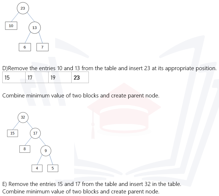
Huffman codes for a:15, e:19, s:5, d:6, f:4, g:7, h:8, t:10

Step 1 Arrange the data in ascending order in a table.

Q2. c) Explain the Partition procedure of the Quick Sort algorithm. Use this procedure and quick sort algorithm to sort the following array of size 8: [12, 9, 17, 15, 23, 19, 16,24]. Compute the worst case and best case complexity of Quick sort algorithm.

Ans) In the Quick Sort algorithm, the partitioning step is crucial as it divides the array into two parts around a pivot element. This partitioning step is essential for the recursive sorting process. The working of partition procedure is as follows:

Choosing a Pivot

The first step in the partition procedure is to select a pivot element from the array. The pivot can be chosen in various ways, such as selecting the first element, the last element, the middle element, or even a randomly chosen element. The choice of pivot can influence the efficiency of the algorithm, especially for special cases like already sorted arrays.

Partitioning Around the Pivot

After selecting the pivot, the array is rearranged such that all elements smaller than the pivot are placed to its left, and all elements greater than the pivot are placed to its right. The pivot itself will be in its final sorted position.

This process is achieved by maintaining two pointers, typically named `i` and `j`, starting from the beginning and the end of the array respectively.

The `i` pointer moves from left to right, and the `j` pointer moves from right to left. At each step, they search for elements that are in the wrong partition (elements that should be on the left side of the pivot but are on the right side, or vice versa).

When `i` finds an element greater than the pivot and `j` finds an element smaller than the pivot, they swap these elements.

This swapping continues until `i` and `j` meet. At this point, all elements smaller than the pivot are on its left, and all elements greater than the pivot are on its right.

Placing the Pivot

Once the `i` and `j` pointers meet, the pivot is placed at its correct sorted position by swapping it with the element pointed to by `i` or `j`.

Now, all elements to the left of the pivot are smaller than the pivot, and all elements to the right of the pivot are greater than the pivot.

Returning the Pivot Index

Finally, the index of the pivot element is returned. This index is important for recursively applying the partition procedure to the subarrays on the left and right of the pivot.

This partitioning step efficiently divides the array into two smaller subarrays, which can then be recursively sorted using the same procedure until the entire array is sorted.

To sort the given array [12, 9, 17, 15, 23, 19, 16, 24] using the Quick Sort algorithm, we'll use the Partition procedure to divide the array into smaller subarrays and recursively sort them.

Step-by-Step Explanation

Choose a pivot element from the array. For simplicity, let's choose the last element (24) as the pivot.

Partition the array such that all elements less than or equal to the pivot are placed to the left, and all elements greater than the pivot are placed to the right.

Recursively apply the Quick Sort algorithm to the subarrays on the left and right of the pivot until the entire array is sorted.

Implementation in Python:

Output:

Sorted array: [9, 12, 15, 16, 17, 19, 23, 24]

Worst-case and best-case complexities of the Quick Sort algorithm

Worst Case Complexity: In the worst-case scenario, the pivot chosen is either the smallest or largest element in the array, leading to highly unbalanced partitions. This results in one subarray with n-1 elements and another with 0 elements. Therefore, the worst-case time complexity of Quick Sort is O(n^2).

Best Case Complexity: In the best-case scenario, the pivot chosen consistently divides the array into two nearly equal halves. This results in balanced partitions, leading to efficient sorting. In the best-case scenario, the time complexity of Quick Sort is O(n log n).

Q2. d) Explain the divide and conquer approach of multiplying two matrices of large size. Also, explain the Strassen's matric multiplication algorithm. Find the time complexity of both these approaches.

Ans) The divide and conquer approach for multiplying two matrices of large size involves breaking down the matrices into smaller submatrices, multiplying these submatrices using recursive calls, and then combining the results to obtain the final product. This approach is particularly useful for large matrices as it reduces the overall number of scalar multiplications required compared to the straightforward iterative method.

Here's a high-level explanation of the divide and conquer approach for matrix multiplication:

Divide: Divide each of the input matrices into smaller submatrices. Typically, this involves partitioning each matrix into quadrants or blocks.

Conquer: Recursively multiply the submatrices obtained from the divide step until the base case is reached. The base case is usually when the submatrices become small enough to be multiplied using a more straightforward algorithm, such as the naive method for small matrices.

Combine: Combine the results of the smaller matrix multiplications to obtain the final product of the original matrices.

Strassen's algorithm is an efficient divide-and-conquer method for multiplying two matrices. It reduces the number of scalar multiplications required compared to the naive method by exploiting the structure of matrix multiplication. The algorithm was introduced by Volker Strassen in 1969.

The key idea behind Strassen's algorithm is to break down the matrix multiplication into a smaller number of subproblems, each involving smaller matrices. By cleverly combining these subproblems, the algorithm achieves a lower asymptotic complexity than the straightforward method.

Here are the high-level steps of Strassen's algorithm:

Divide: Given two matrices A and B of size n × n, divide each matrix into four equal-sized submatrices of size n/2 × n/2. This step involves dividing the matrices into quadrants.

Conquer: Recursively compute seven matrix products using the submatrices obtained in the previous step:

Compute the following submatrix products:

P1 = (A11 + A22) * (B11 + B22)

P2 = (A21 + A22) * B11

P3 = A11 * (B12 - B22)

P4 = A22 * (B21 - B11)

P5 = (A11 + A12) * B22

P6 = (A21 - A11) * (B11 + B12)

P7 = (A12 - A22) * (B21 + B22)

Each of these products involves matrix additions and subtractions.

Combine: Compute the resulting submatrices C11, C12, C21, and C22, which form the final product matrix C:

C11 = P1 + P4 - P5 + P7

C12 = P3 + P5

C21 = P2 + P4

C22 = P1 - P2 + P3 + P6

Base Case: If the size of the matrices becomes small enough (typically a threshold value), switch to a base case method such as the naive method for matrix multiplication.

The Divide and Conquer algorithm solves the problem in O(N log N) time.

Strassen’s Algorithm is an efficient algorithm to multiply two matrices. A simple method to multiply two matrices needs 3 nested loops and is O(n^3). Strassen’s algorithm multiplies two matrices in O(n^2.8974) time.

Q2. e) What is the use of Topological sorting? Write and explain the Topological sorting algorithm. Also, compute the time complexity for the topological sorting algorithm.

Ans) Topological sorting is a technique used in graph theory to order the vertices of a directed graph in such a way that if there is a directed edge from vertex A to vertex B, then vertex A comes before vertex B in the ordering. This ordering is useful in various applications such as task scheduling, dependency resolution, and determining the order of execution in a directed acyclic graph (DAG).

Topological sorting algorithm typically works as follows:

1. Initialize: Begin by initializing an empty list to store the sorted vertices and a set or array to keep track of visited vertices.

2. Visit Unvisited Vertices: Iterate through each vertex in the graph. For each unvisited vertex encountered, call a depth-first search (DFS) or breadth-first search (BFS) function to explore its neighbours.

3. DFS/BFS Traversal: During the traversal, recursively visit each neighbour of the current vertex. Mark each visited vertex as visited to avoid revisiting it.

4. Backtrack and Add to the Sorted List: After visiting all neighbours of a vertex, backtrack and add the current vertex to the sorted list. This ensures that vertices are added to the sorted list in the correct order based on their dependencies.

5. Finalize: Once all vertices have been visited and added to the sorted list, return the list as the result of the topological sorting.

Example

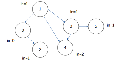
Here, "in"=indegree

Order of removal : First 0, then 1 and 2, then 3 and finally 4 and 5

Topological order: 0, 1, 2, 3, 4, 5

The key operations involved in topological sorting are:

Visiting each vertex in the graph once.

Visiting each edge in the graph once.

Assuming the graph has V vertices and E edges.

Visiting each vertex in the graph: In the worst case, every vertex will be visited once. This operation has a time complexity of O(V).

Visiting each edge in the graph: In the worst case, every edge will be visited once. Since we are using an adjacency list representation for the graph, visiting all edges connected to a vertex may take O(E) time overall.

Hence, the overall time complexity of the topological sorting algorithm using depth-first search (DFS) is O(V + E).

Q3) Consider the following Graph:

a) Write the Kruskal's algorithm and Prim's algorithm to find the minimum cost spanning tree of the graph given in Figure l. Show all the steps of computation. Also, compute the time complexity of both the algorithms.

Ans) Kruskal’s algorithm is an algorithm to find the minimum cost spanning tree (MST) in a connected graph. Kruskal’s algorithm finds a subset of a graph G such that:

It forms a tree with every vertex in it.

The sum of the weights is the minimum among all the spanning trees that can be formed from this graph.

The sequence of steps for Kruskal’s algorithm is as follows:

First sort all the edges from the lowest weight to highest.

Take edge with the lowest weight and add it to the spanning tree. If the cycle is created, discard the edge.

Keep adding edges like in step 1 until all the vertices are considered.

Below is the illustration of the algorithm:

We have a spanning tree with minimum cost.

Prim’s algorithm is yet another algorithm to find the minimum spanning tree of a graph. In contrast to Kruskal’s algorithm that starts with graph edges, Prim’s algorithm starts with a vertex. We start with one vertex and keep on adding edges with the least weight till all the vertices are covered.

The sequence of steps for Prim’s Algorithm is as follows:

a. Choose a random vertex as starting vertex and initialize a minimum spanning tree.

b. Find the edges that connect to other vertices. Find the edge with minimum weight and add it to the spanning tree.

c. Repeat step 2 until the spanning tree is obtained.

This is the spanning tree with minimum cost.

Time complexity of Kruskal's Algorithm:

Kruskal's algorithm sorts all the edges of the graph based on their weights and then selects the edges in ascending order of weight while ensuring that no cycle is formed. It typically uses a disjoint-set data structure (such as Union-Find) to keep track of which vertices are connected. The time complexity of Kruskal's algorithm depends on the sorting step and the disjoint-set operations.

Sorting the edges: O(E log E) or O(E log V), where E is the number of edges and V is the number of vertices.

Union-Find operations (for each edge): O(log V).

Total time complexity: O(E log E + E log V) or O(E log V).

Time complexity of Prim's Algorithm:

Prim's algorithm starts from an arbitrary vertex and grows a single tree by iteratively adding the shortest edge that connects the tree to a vertex not yet in the tree. It typically uses a priority queue to efficiently select the minimum-weight edge at each step.

Priority queue operations (insertion and extraction of minimum): O(log V).

Total time complexity: O(E log V).

Q3. b) In the Figure 1, find the shortest path from the vertex 'a' using Dijkstra's shortest path algorithm. Show all the steps of computation. Also, find the time complexity of the algorithm.

Ans) Dijkstra's algorithm is an algorithm for finding the shortest paths between nodes in a weighted graph, which may represent, for example, road networks.

The sequence of steps for Dijkstra’s shortest path algorithm is as follows:

1. Mark the source node with a current distance of 0 and the rest with infinity.

2. Set the non-visited node with the smallest current distance as the current node.

3. For each neighbour, N of the current node adds the current distance of the adjacent node with the weight of the edge connecting 0->1. If it is smaller than the current distance of Node, set it as the new current distance of N.

4. Mark the current node 1 as visited.

5. Go to step 2 if there are any nodes are unvisited.

Illustration

Dijkstra algorithm is a type of greedy algorithm. It only works on weighted graphs with positive weights. It has a time complexity of 0( V2) using the adjacency matrix representation of graph. The time complexity can be reduced to0((V + E) log V) using adjacency list representation of graph, where E is the number of edges in the graph and V is the number of vertices in the graph.

Q3. c ) What is dynamic programming? What is the principle of Optimality? Use the dynamic programming approach to find the optimal sequence of chain multiplication of the following matrices:

Ans) Dynamic programming is a method for solving complex problems by breaking them down into simpler subproblems and solving each subproblem only once. It's particularly useful for optimization problems where you are trying to maximize or minimize some value. The key idea behind dynamic programming is to store the solutions of subproblems so that they don't need to be recomputed every time they are encountered.

The principle of Optimality, often associated with dynamic programming, states that an optimal solution to a problem contains within it optimal solutions to its subproblems. In other words, if you can find the optimal solution to a larger problem by combining optimal solutions to its smaller subproblems, then the problem exhibits the principle of Optimality.

This principle enables dynamic programming algorithms to work efficiently by avoiding redundant calculations. Instead of solving the same subproblems repeatedly, dynamic programming algorithms solve each subproblem once and store its solution for future reference, reducing the time complexity of the overall algorithm.

Steps to find the optimal sequence of chain multiplication of the given matrices using dynamic programming are:

Define the subproblems: We can define the subproblems as finding the optimal sequence of multiplication for sub chains of matrices.

Formulate the recursive relation: We'll use dynamic programming to compute the minimum number of scalar multiplications needed to compute the product of matrices from i to j, where i and j are indices representing the matrices.

Use memoization or bottom-up approach: We'll either use memoization to store the results of subproblems or use a bottom-up approach to iteratively solve them.

Python implementation using bottom-up dynamic programming:

import sys

def matrix_chain_order(dimensions):

n = len(dimensions)

# Initialize a table to store the minimum number of scalar multiplications

dp = [[0] * n for _ in range(n)]

# Chain length is 1, so cost is 0

for i in range(n):

dp[i][i] = 0

# Chain length from 2 to n

for chain_length in range(2, n + 1):

for i in range(n - chain_length + 1):

j = i + chain_length - 1

dp[i][j] = sys.maxsize # Initialize to maximum possible value

for k in range(i, j):

# Cost of multiplication

cost = dp[i][k] + dp[k + 1][j] + dimensions[i][0] dimensions[k][1] dimensions[j][1]

dp[i][j] = min(dp[i][j], cost)

return dp[0][n - 1]

# Define dimensions of matrices

dimensions = [(5, 10), (10, 20), (20, 15), (15, 8), (8, 10)]

# Calculate the optimal number of scalar multiplications

optimal_multiplications = matrix_chain_order(dimensions)

print("Minimum number of scalar multiplications:", optimal_multiplications)

Q3. d) Make all the possible Binary Search Trees for the key values 25, 50, 75.

Ans) For N = 3, there are 5 possible BSTs

Q 3. e) Explain the Knuth Morris Pratt algorithm for string matching. Use this algorithm

to find a pattern “algo” in the Text “From algae to algorithms”. Show all the steps.

What is the time complexity of this algorithm.

Ans) The Knuth-Morris-Pratt (KMP) algorithm is a string matching algorithm that efficiently finds occurrences of a pattern within a text. It is particularly efficient for large texts where traditional brute-force methods become slow. The key idea behind the KMP algorithm is to avoid unnecessary character comparisons by utilizing information about the pattern itself.

KMP Algorithm Explanation:

Preprocessing (Building the Prefix Function):

Construct the prefix function (also known as the failure function) for the pattern. This function helps in determining the maximum length of the proper suffix of the pattern that is also a prefix. It is used to efficiently shift the pattern during the matching process.

Matching:

- Iterate through the text and the pattern simultaneously.

- Compare characters of the text and the pattern:

- If they match, move both pointers forward.

- If they don't match:

- Utilize the information from the prefix function to determine the next position to start comparing from in the pattern (rather than starting from the beginning).

- Adjust the pattern pointer accordingly and continue comparing.

Example: Finding "algo" in "From algae to algorithms

Compute the Prefix Function for the Pattern:

For the pattern "algo", the prefix function is [0, 0, 0, 0] since there are no proper prefixes that are also suffixes.

Search for the Pattern in the Text:

We start with q = 0 and i = 0.

Compare the first character of the pattern ("a") with the first character of the text ("F"). They do not match, so we move to the next character in the text.

Repeat this process until we find a match or reach the end of the text.

When we reach "a" in "algorithms" (index 15), we have a match.

Result:

The pattern "algo" is found starting at index 15 in the text "From algae to algorithms".

Time Complexity

The KMP is the only string-matching algorithm with a time complexity of O(n+m), where n is the string length and m is the pattern length.

Q4. a) What are decision problems and Optimisation problems? Differentiate the decision problems and Optimisation problems with the help of at least two problem statements of each.

Ans)

Decision Problems

Decision problems are computational problems where the answer is either yes or no, true or false, 1 or 0. These problems require determining whether a given input satisfies a certain property or condition. The goal is to make a binary decision based on the input data.

Optimization Problems

Optimization problems involve finding the best solution among a set of feasible solutions. Instead of just determining whether a solution exists, optimization problems seek to find the optimal solution that maximizes or minimizes an objective function, subject to constraints.

Difference between Decision Problems and Optimization Problems:

Decision Problems:

These problems involve determining whether a certain condition or property holds for a given input. The answer to a decision problem is typically "yes" or "no".

Problem Statement 1 (Graph Connectivity):

- Given an undirected graph G and two vertices u and v, determine whether there exists a path from u to v in G.

- Decision: Is there a path from vertex u to vertex v in graph G?

Problem Statement 2 (Integer Factorization):

- Given a positive integer n, determine whether it has any divisors other than 1 and itself.

- Decision: Is n a prime number?

Optimization Problems: These problems involve finding the best solution from all feasible solutions according to a certain criterion, often maximizing or minimizing an objective function.

Problem Statement 1 (Traveling Salesman Problem):

Given a list of cities and the distances between each pair of cities, find the shortest possible route that visits each city exactly once and returns to the original city.

Optimization: Find the shortest Hamiltonian cycle in a complete weighted graph.

Problem Statement 2 (Knapsack Problem):

Given a set of items, each with a weight and a value, determine the most valuable combination of items that can be carried with a weight constraint.

Optimization: Maximize the total value of items selected without exceeding the weight capacity of the knapsack.

Q4. b) Define P and NP class of Problems with the help of examples. How are P class of problem different from NP class of Problems.

Ans) P Class of Problems

The class P (polynomial time) consists of decision problems that can be solved by a deterministic Turing machine in polynomial time, where the time taken by the algorithm is bounded by a polynomial function of the size of the input.

Example of a P Problem

Sorting: Given a list of elements, sorting them in ascending or descending order can be done in polynomial time. Algorithms like Quicksort, Mergesort, and Heapsort all have worst-case time complexities of O(nlogn), which is polynomial in the size of the input list.

NP Class of Problems

The class NP (nondeterministic polynomial time) consists of decision problems for which a given solution can be verified in polynomial time by a deterministic Turing machine. In other words, if someone presents a potential solution, we can quickly check if it's correct.

Example of an NP Problem

Graph Hamiltonian Path:: Given a graph G and two vertices s and t, an NP problem would be to determine whether there exists a path that visits every vertex in the graph exactly once and starts at s and ends at t. If someone presents such a path, we can verify in polynomial time that it indeed satisfies the conditions.

Difference between P and NP

The main difference between P and NP problems lies in the nature of their solutions.

P Problems: Problems in P can be solved efficiently by algorithms in polynomial time.

NP Problems : Problems in NP may not necessarily be efficiently solvable, but if we are given a potential solution, we can efficiently verify its correctness.

Q4. c) What are NP-Hard and NP-Complete problem? What is the role of reduction? Explain with the help of an example.

Ans)

NP-Hard Problems

These are decision problems that are at least as hard as the hardest problems in NP (nondeterministic polynomial time).

NP-Hard problems don't have to be in NP; they only need to be as hard as the problems in NP.

They don't necessarily have a polynomial-time algorithm for verification, but any problem in NP can be reduced to an NP-Hard problem in polynomial time.

Solving an NP-Hard problem in polynomial time would imply that P (polynomial time) equals NP, which is an unresolved question in computer science.

NP-Complete Problems

These are the hardest problems in NP; they are both in NP and NP-Hard.

If any NP-Complete problem can be solved in polynomial time, then all problems in NP can also be solved in polynomial time.

NP-Complete problems are essentially the "most difficult" problems within NP.

Finding a polynomial-time algorithm for any NP-Complete problem would prove P = NP.

Role of Reduction

Reduction is a technique used to show that one problem is at least as hard as another.

In the context of NP-Completeness, polynomial-time reduction is often used.

If Problem A can be reduced to Problem B in polynomial time and Problem B is NP-Hard, then Problem A is at least as hard as Problem B and is also NP-Hard.

This establishes a relationship between the difficulty of different problems.

Example

Consider the traveling salesman problem (TSP) and the Hamiltonian cycle problem (HAM-CYCLE):

Traveling Salesman Problem (TSP): Given a list of cities and the distances between each pair of cities, find the shortest possible route that visits each city exactly once and returns to the original city.

Hamiltonian Cycle Problem (HAM-CYCLE): Given a graph, determine whether there is a cycle that visits every vertex exactly once.

Now, we can show that HAM-CYCLE is NP-Complete by reducing TSP to HAM-CYCLE:

Given an instance of TSP, construct a graph where cities are vertices and distances between cities are edges.

Now, if we have a Hamiltonian cycle in this graph, we can simply traverse this cycle, which will give us a solution to TSP.

Therefore, TSP reduces to HAM-CYCLE in polynomial time.

Since TSP is known to be NP-Hard, and we have shown a polynomial-time reduction from TSP to HAM-CYCLE, HAM-CYCLE must also be NP-Hard.

Since HAM-CYCLE is also in NP, it is NP-Complete.

This example illustrates how reduction is used to establish the complexity of a problem by relating it to a known NP-Hard problem.

Q4. d) Define the following Problems:

(i) 3-CNF SAT

Ans) CNF SAT refers to the problem of determining whether a given Boolean formula, expressed in conjunctive normal form (CNF), can be satisfied by assigning truth values to its variables in such a way that the entire formula evaluates to true.

(ii) Clique problem

Ans) The Clique Problem is a computational problem in graph theory that seeks to find the largest complete subgraph, or clique, within a given graph. A clique in a graph is a subset of vertices where every pair of vertices is connected by an edge. In other words, in a clique, every vertex is directly connected to every other vertex in the subset.

(iii) Vertex cover problem

Ans) The Vertex Cover Problem is a fundamental problem in graph theory and combinatorial optimization. It involves finding the smallest set of vertices in a graph such that every edge in the graph is incident to at least one vertex in the set.

(iv) Graph Colouring Problem

Ans) The Graph Colouring Problem is a classic problem in graph theory and combinatorial optimization. It involves assigning colours to the vertices of a graph such that no two adjacent vertices share the same colour, while using as few colours as possible.