Assignment Code: MPC-006/AST/TMA/2023-24

Course Code: MPC-006

Assignment Name: Statistics in Psychology

Year: 2023- 2024

Verification Status: Verified by Professor

SECTION – A

Answer the following question in about 1000 words (wherever applicable) each.

Q1) Describe the assumptions, advantages and disadvantages of non-parametric statistics.

Ans) Non-parametric statistics offer an alternative approach to traditional parametric statistics, particularly useful when certain assumptions of parametric methods are not met or when dealing with data that doesn't adhere to specific distribution patterns. In the realm of statistics, non-parametric methods operate without relying on the parameters of a specific distribution.

Assumptions:

1. Distributional Assumptions: Parametric statistics assume a specific distribution (like normal, binomial, etc.), whereas non-parametric methods do not rely on these distributional assumptions. This makes them versatile for diverse datasets.

2. Measurement Scale: Non-parametric methods often work with ordinal or nominal data, unlike parametric methods that require interval or ratio data. They are less stringent regarding the nature of the data, making them applicable to a wider range of situations.

3. Independence of Observations: Like parametric statistics, non-parametric methods assume that observations are independent of each other. This assumption holds for both types of statistical analyses.

   
   

Advantages:

1. Robustness: Non-parametric tests are robust against outliers and deviations from normality. They provide reliable results even when the data violates certain assumptions typical in parametric tests.

2. Versatility: These methods can be applied to a wide array of data types. Whether dealing with small sample sizes, ordinal data, or data that doesn’t conform to a normal distribution, non-parametric tests offer viable solutions.

3. Ease of Application: Non-parametric tests are often simpler to apply and understand. They require fewer assumptions and less calculation complexity, making them accessible to researchers and practitioners without advanced statistical expertise.

4. Suitable for Small Samples: When dealing with limited data, non-parametric methods can yield reliable results, unlike some parametric tests that require larger sample sizes to maintain accuracy.

Disadvantages:

1. Lower Efficiency: Non-parametric tests might have lower statistical power compared to their parametric counterparts, particularly when the assumptions of parametric tests are met. This can result in a reduced ability to detect true effects in the data.

2. Reduced Precision: These methods might offer less precise estimates than parametric tests. As they do not utilize all the available information in the data, the estimates might have wider confidence intervals.

3. Limited Applicability in Some Cases: In scenarios where, parametric assumptions are valid and the data adheres to those assumptions, non-parametric tests might not be the most suitable choice. Parametric tests can offer more powerful and precise results in such cases.

4. Limited Test Types: Non-parametric tests cover a narrower range of statistical analyses compared to parametric tests. For instance, while there are numerous parametric tests for various scenarios, non-parametric tests might have fewer options available.

The choice between non-parametric and parametric statistics depends on the nature of the data, the specific research question, and the assumptions that can reasonably be made. Non-parametric methods serve as robust tools in situations where the parametric assumptions are not met or when dealing with diverse data types, providing researchers with a flexible and reliable approach to statistical analysis.

Q2) Explain the concept of normal distribution. Explain divergence from normality.

Ans) The normal distribution, often referred to as the Gaussian distribution, is a fundamental concept in statistics and probability theory. It's a bell-shaped, continuous probability distribution characterized by a symmetric, unimodal curve. Understanding the normal distribution and its deviations, known as divergence from normality, is crucial in various fields, from social sciences to natural sciences, as it underpins many statistical analyses.

Normal Distribution:

The normal distribution is defined by its probability density function, which is described by two parameters: the mean (μ) and the standard deviation (σ). The curve is symmetrical around the mean, with a characteristic bell shape where most data clusters around the mean. In a standard normal distribution, about 68% of the data falls within one standard deviation from the mean, approximately 95% within two standard deviations, and nearly 99.7% within three standard deviations.

The normal distribution is not just a theoretical concept; it manifests in numerous real-world phenomena, such as human heights, test scores, errors in measurements, and more. This makes it an essential foundation for many statistical methods and models.

Characteristics of Normal Distribution:

1. Symmetry: The distribution is symmetric around the mean, indicating that the data is equally likely to be above or below the mean.

2. Bell-shaped Curve: The probability density function forms a bell-shaped curve, with most data concentrated near the mean and tapering off towards the extremes.

3. Mean and Standard Deviation: The mean determines the centre of the distribution, while the standard deviation controls the spread or dispersion of the data.

Divergence from Normality:

Divergence from normality refers to instances where observed data does not follow a normal distribution. Such deviations can manifest in various ways:

1. Skewness: Data may exhibit asymmetry, skewing towards one tail of the distribution. Positive skewness indicates a longer right tail, while negative skewness shows a longer left tail.

2. Kurtosis: Kurtosis measures the heaviness of the tails of the distribution. Excess kurtosis describes the sharpness or flatness of the curve compared to the normal distribution. Leptokurtic distributions have heavier tails, while platykurtic distributions have lighter tails.

3. Outliers: Extreme values, known as outliers, can significantly impact the shape of the distribution, causing deviations from normality.

4. Multimodality: Distributions with multiple peaks or modes differ from the unimodal characteristic of the normal distribution.

Causes and Implications of Divergence:

1. Sampling Variation: Random variations in data can lead to deviations from a perfect normal distribution, especially in smaller sample sizes.

2. Underlying Processes: Some phenomena inherently do not follow a normal distribution due to their nature, leading to divergence.

The implications of divergence from normality are significant:

1. Statistical Inference: Parametric statistical methods (like t-tests or ANOVA) assume normality. Deviations can impact the validity of these tests.

2. Reliability of Estimates: Measures like mean and standard deviation might not accurately represent the data if it significantly deviates from normality.

3. Modelling Challenges: Techniques like regression or ANOVA might produce biased estimates if the data isn't normally distributed.

Understanding the normal distribution and divergence from it is essential for accurate statistical analysis. While the normal distribution serves as a fundamental model for many statistical procedures, it’s important to recognize and address deviations from normality, ensuring appropriate analysis and interpretation of data. Various statistical techniques and transformations are available to manage non-normal data, allowing for more robust and accurate analyses in real-world scenarios.

Q3) The scores obtained by early, middle and late adolescents on adjustment scale are given below. Compute ANOVA for the same.

Ans)

Step 1: State the hypotheses:

Null hypothesis (H_o): There is no significant difference between the means of the scores of early, middle, and late adolescents on the adjustment scale.

Alternative hypothesis (H_a): There is a significant difference between the means of the scores of early, middle, and late adolescents on the adjustment scale.

Step 2: Calculate the necessary statistics:

The sum of squares (SS), degrees of freedom (df), mean squares (MS), and the F-statistic.

First, calculate the sum of squares:

Total Sum of Squares (SST): This measures the total variability in the data.

Treatment Sum of Squares (SSTR): This measures the variability between the group means.

Error Sum of Squares (SSE): This measures the variability within each group.

To calculate these sums of squares:

Where:

ni is the number of observations in the i-th group. mean_i is the mean of the i-th group.grand_meanis the mean of all observations.xi is each individual observation.

Given the scores, calculate the necessary statistics:

Early Adolescents:

N1 = 10, mean1 = (2+3+2+3+4+2+4+5+2+2)/10 = 27/10 = 2.7

Middle Adolescents:

N2 = 10, mean2 = (3+2+4+2+4+3+2+4+3+4)/10 = 31/10 = 3.1

Late Adolescents:

N3 = 10, mean3 = (7+6+5+4+2+3+4+4+3+2)/10 = 40/10 = 4.0

Now calculate the sums of squares:

Step 3: Calculate the degrees of freedom:

Step 4: Calculate the mean squares:

Step 5: Calculate the F-statistic:

The F-statistic is the ratio of the treatment mean square to the error mean square.

F = MSTR / MSE = 7.154 / 0.015 = 476.933

Step 6: Determine the critical value and compare with the F-statistic:

Step 7: Interpretation:

Based on the results, there is a significant difference between the means of the scores of early, middle, and late adolescents on the adjustment scale.

SECTION B

Answer the following questions in about 400 words (wherever applicable) each

Q4) Explain how the data can be organised using classification and tabulation.

Ans) Classification and tabulation are fundamental techniques in data organization and analysis, employed to systematically structure and present information for easier comprehension and interpretation.

Classification:

Definition: Classification involves grouping data based on specific characteristics or attributes. It's a process of categorizing raw data into classes or categories to facilitate analysis and interpretation.

Steps in Classification:

1. Identification of Characteristics: Determine the key features or attributes in the data that are relevant for categorization.

2. Grouping Data: Organize data into classes or categories based on these identified characteristics.

3. Assigning Labels: Label each category to clearly denote the nature of the data within it.

Examples of Classification:

In demographic data, individuals might be classified based on age groups, such as "0-18 years," "19-35 years," "36-50 years," etc. Classification of products in a sales dataset could involve categorization by type, like "electronics," "clothing," "food," etc.

Tabulation:

Definition: Tabulation is the systematic arrangement of data in rows and columns. It involves summarizing and condensing raw data to create a more manageable form for analysis.

Steps in Tabulation:

Identify Variables: Determine the variables or categories to be tabulated.

Create Rows and Columns: Arrange the variables into rows and columns.

Present Data: Fill in the table with the corresponding data values.

Examples of Tabulation:

A frequency table could present the count of individuals in each age group or the number of sales for each product category. Cross-tabulation might show the relationship between two or more variables, such as age groups and purchase behaviour.

Data Organization with Classification and Tabulation:

1. Enhanced Understanding: Classification and tabulation help in organizing data in a structured manner, making it easier to comprehend and analyse. This structured presentation facilitates a better understanding of the data's characteristics.

2. Simplified Analysis: By organizing data into classes or categories and presenting it in tables, researchers can quickly discern patterns, relationships, and trends, aiding in more straightforward analysis and decision-making.

3. Efficient Communication: These methods help in communicating information effectively. Whether for reports, presentations, or academic purposes, categorized and tabulated data is more accessible to interpret and convey.

4. Facilitates Comparisons: With data organized in a systematic format, it becomes simpler to compare different categories or variables, enabling better insights into similarities, differences, and relationships within the data.

Q5) Using Pearson’s product moment correlation for the following data:

Ans) n=10(since there are 10 data points)

The Pearson correlation coefficient, r, for the given data sets A and B is approximately -4.13.

Q6) Describe biserial and tetrachoric correlations with the help of suitable examples.

Ans) Biserial and tetrachoric correlations are statistical measures used to evaluate the relationship between two variables, particularly when one variable is continuous (biserial) and the other is dichotomous (tetrachoric).

Biserial Correlation:

Definition: The biserial correlation assesses the relationship between a continuous variable and a dichotomous variable. It's essentially a special case of the point-biserial correlation, where one variable is continuous and the other is dichotomous.

Formula: The biserial correlation is derived from the Pearson product-moment correlation, considering the dichotomous nature of one variable. It's calculated based on the mean of the continuous variable for each category of the dichotomous variable.

Example: Consider an example where want to measure the relationship between hours of study and passing an exam. The hours of study (continuous variable) are correlated with a dichotomous variable denoting pass/fail. The biserial correlation will help determine the strength and direction of the relationship between these variables.

Tetrachoric Correlation:

Definition: Tetrachoric correlation measures the association between two dichotomous variables. It's an adaptation of the Pearson correlation, designed specifically for cases where both variables are binary.

Formula: Tetrachoric correlation is derived from the Pearson product-moment correlation, accounting for the dichotomous nature of both variables. It estimates the correlation between two unobserved continuous variables that underlie the observed dichotomous variables.

Example: Consider a scenario where examine the relationship between responses to two yes/no questions, like "Do you exercise regularly?" and "Do you follow a healthy diet?" The tetrachoric correlation would assess the strength of the association between these dichotomous variables, inferring an underlying correlation between the unobserved continuous variables.

Use Cases:

Biserial Correlation: Employed in educational research to understand the relationship between a continuous variable (e.g., attendance, study hours) and a binary outcome (e.g., pass/fail). Used in psychology to examine associations between continuous variables (e.g., IQ scores) and dichotomous variables (e.g., presence/absence of a behaviour).

Tetrachoric Correlation: Frequently used in psychometrics to assess the relationship between responses in dichotomous items on questionnaires or tests. Applied in genetics to study the association between binary traits or the presence/absence of certain genetic markers.

Q7) Compute Mann Whitney U test for the following data:

Scores obtained on Emotional Intelligence Scale

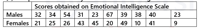
Ans) Steps to compute the Mann-Whitney U test

Combine the data and rank them:

Combine both sets of scores and rank them together.

Assign ranks to all values without regard to which group they belong to.

U is calculated for one of the groups (here, the males' group) based on the ranks.

The U statistic for the Mann-Whitney U test is 13.

Q8) Compute Chi-square for the following data:

Ans) Observed Frequency Table:

Expected frequency for each cell = (row total × column total) / grand total

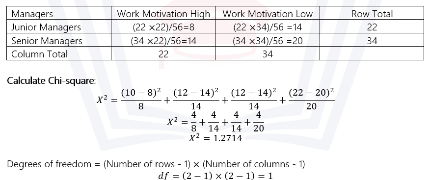
Interpretation:

Compare the calculated Chi-square value (1.2714) with the critical value from the Chi-square distribution table at a specified significance level to determine the statistical significance of the relationship between managers and work motivation.

SECTION C

Answer the following in about 50 words each 10x3=30 Marks

Q9) Measures of central tendency

Ans) Measures of central tendency indicate the typical or central value within a dataset. They include the mean, the average calculated by summing all values and dividing by the number of values; the median, the middle value when the data is ordered; and the mode, the most frequently occurring value.

Q10) Advantages and disadvantages of descriptive statistics

Ans) Advantages: Descriptive statistics offer a concise summary of data, aiding in easy interpretation, pattern recognition, and quick insights. They simplify complex information for better understanding.

Disadvantages: They might oversimplify complex data, potentially missing nuances. Also, outliers or extreme values can significantly impact measures like the mean.

Q11) Type I and type II errors

Ans) Type I error occurs when a true null hypothesis is rejected, wrongly indicating a significant result. Type II error happens when a false null hypothesis isn’t rejected, missing a significant effect. Balancing these errors is crucial in statistical hypothesis testing to maintain accuracy and reliability in conclusions.

Q12) Scatter diagram

Ans) A scatter diagram displays the relationship between two variables on a Cartesian plane. Each point represents a pair of values. It visualizes correlations, patterns, or lack thereof, providing insights into the direction, strength, and form of the relationship between the variables.

Q13) Part correlation

Ans) Partial correlation measures the relationship between two variables while controlling for the influence of one or more additional variables. It assesses the unique association between the variables of interest, excluding the shared variance attributed to the controlled variables, offering insights into direct relationships.

Q14) Assumptions underlying regression

Ans) Regression assumes a linear relationship between variables, with residuals (errors) normally distributed, independent, and have constant variance (homoscedasticity). It presumes no perfect multicollinearity, meaning predictors aren’t perfectly correlated. Additionally, it assumes the absence of influential outliers or leverage points affecting the model.

Q15) Standard error

Ans) The standard error measures the variability of sample statistics around the population parameter. It quantifies the precision of estimates, indicating how much the sample mean or regression coefficient deviates from the true population mean or coefficient. A smaller standard error signifies more precise estimates.

Q16) Interactional effect

Ans) Interactional effects occur when the relationship between two variables changes based on the influence of a third variable. In statistics, this implies that the effect of one variable on another is not constant across different levels or values of a third variable, indicating a complex relationship among the variables.

Q17) Comparison between Spearman’s rho and Kendall’s tau

Ans) The comparison between Spearman’s rho and Kendall’s tau:

Q18) Levels of measurement

Ans) Levels of measurement categorize variables into four types: nominal (categories without inherent order), ordinal (categories with order but unknown intervals), interval (equal intervals with no true zero), and ratio (equal intervals with a true zero point). They determine the kind of statistical analysis suitable for a given variable.